前言
笔者在老虎书 “Fundamentals of Computer Graphics” 的第四章 "RayTracing" 中学习到了光线追踪的理论基础,并根据书上的理论自己实现了一个简易的光线追踪算法。借此篇记录算法实现上的一些要点。
如对文章的内容有疑惑或有错误指出,欢迎在评论区留言
目录
什么是光线追踪光线追踪算法概述生成初始光线光线与物体相交光线反射着色模型代码详解结果展示与总结参考文献
什么是光线追踪
要解释光线追踪首先需要解释光线是如何成像的。以摄影为例,摄影形成照片的过程可以简化为:光源会向四周发出无数光线,若光线的传播路径上存在物体,则光线会在相交后产生反射或折射,并沿反射方向射出,光源发出的一部分光线会经过多次反射后最终落在相机的感光底片中。底片接收到的光线总和构成了最终的拍摄出来的图像。
可以说,摄影的成像是把三维的场景映射到二维图像中。计算机成像与摄影成像类似,但计算机无法模拟现实中摄影成像的过程,因为哪怕是一个最小的光源都能向全方位发出无数的光线,要求计算机跟踪并计算出每一条光线最终的落点是一项不可能实现的任务。
但参与成像的光线的数量是有限并可知的,因为成像面的大小是固定的,每个像素点对应一条光线,则光线数等于像素数。如果把摄影成像的过程倒转过来,不是从光源出发计算落点,而是从成像面出发,逆推光线的路径,直到回溯到光源,就能逆向模拟成像过程。虽然这样做的计算量大,但却是当今计算机能够承受的。而这一个过程,就被称作“光线追踪 (Ray Tracing)”。
以下图的场景为例。下图用1024*768个像素渲染了一个三维场景。光源位于顶部,左侧球体为镜面材质,右侧球体为玻璃材质。假设对左侧小球上黄点所处位置的像素进行光线追踪,光线首先从黄点所处位置的像素出发,落在左边的球体上,经过反射落在左边红色的墙上的蓝点处,最后再次反射到顶部的光源中,由于球体是镜面材质,球体会完全反射墙面的颜色,因此黄点处像素的颜色与左侧墙的颜色一致。光线追踪路径如下图箭头所示:
Figure 1: 1024*768全域光渲染器效果图
光线追踪算法概述
根据上文所述的光线追踪原理,我们可以推导出光线追踪的建议框架,总结成伪代码就是:
for each pixel do :compute viewing rayif (ray hits an object) then :get hit object IDcompute reflected ray evaluate shading modelrecursively trace ray back until stopset pixel to shading colorelse :set shading color to background color
大致流程为:
生成初始光线
要生成光线,光线的数学表达式是必须具备的。光线是由光源产生的有向射线。基于这个原理,任意光线在数学上均可由光线的源点及光线的传播方向来表示。可得如下公式:
P(t)⃗=e⃗+t⋅d⃗t∈(0,∞)(1)\vec{P(t)} = \vec{e} + t \cdot \vec{d} \qquad t\in(0,\infty) \tag{1}P(t)=e+t⋅dt∈(0,∞)(1)
其中 e⃗\vec{e}e 为光线源点的三维坐标,d⃗\vec{d}d 为光线的方向单位向量,ttt 是一个标量,表示沿 d⃗\vec{d}d 方向上到源点的距离。整个公式表示的是光线路径上与源点距离为 ttt 的一个点,而光线路径上所有点的总集构成了光线本身。
在具备了光线的数学表达式后,便可计算初始光线的位置和方向,但这两者的数值都不是随便设定的,计算这两者的数值牵涉到另一位问题,即视角问题。
在计算机图形学领域中,主要有两种视角,即正交视角(Orthographic View,也被称为Parallel View)和透视视角(Perspective View)。在正交视角下,物体的成像是以垂直于成像面的方式映射在对应的像素点上,因此所有初始光线的方向均相同且垂直于成像面,而起始点则在各自对应的成像面像素点上。
而透视视角更贴近于人眼的成像,所有初始光线的均由一个点发出,通常这个点被称作视点(Viewing Point),而成像面则位于视点前,所有的初始光线由视点出发,再经过其对应的成像面像素点。因此在透视视角下,光线的方向是各不相同且呈现出辐射状的分布。两种视角下初始光线的差异可见下图的比较:
Figure 2: 正交视角和透视视角的对比
因此对于任意一个像素点 p⃗=(x,y,z)\vec{p}=(x,y,z)p=(x,y,z) 来说,正交视角下的初始光线可以表达为:
ray.position=p⃗ray.position = \vec{p}ray.position=p ray.direction=−w⃗(2)ray.direction = -\vec{w} \tag{2}ray.direction=−w(2)
透视视角下的初始光线可以表达为:
ray.position=e⃗ray.position = \vec{e}ray.position=e ray.direction=−d∗w⃗+x∗u⃗+y∗v⃗ray.direction = -d*\vec{w} \ + \ x*\vec{u} \ + \ y*\vec{v}ray.direction=−d∗w+x∗u+y∗v
其中,p⃗\vec{p}p 为像素点的三维坐标,u⃗,v⃗,w⃗\vec{u} ,\ \vec{v} ,\ \vec{w}u,v,w 分别为基于成像面建立的坐标系,向右、向上,向外的单位向量。e⃗\vec{e}e 是视点的三维坐标,ddd 是视点到成像面的距离。
为了方便计算,本篇博客所分享的算法采用的是正交视角。
光线与物体相交
光线追踪第二个需要解决的问题是判断光线是否与空间中物体存在相交关系。同样地,我们需要建立物体在三维空间中的数学表达式才能进一步对其进行计算。
在当前计算机图形学领域中,光线与物体的相交处理主要集中在球体和三角面上。球体这个好理解,但为何会选用三角面呢?三角面是三维平面的所有数学表达中最轻量的表达,任意多变面均可由若干三角面组成。以此类推,三维空间中的任意物体(实际上也包括球体)均可由多个三角面来组成,即通过组合三角面,我们可以得到空间中任意的物体。
但一些精细的模型往往会有上千甚至上万个三角面,要对这样一个物体进行光线追踪将会消耗大量的时间和算力。本文图一中的场景就是渲染了10+个小时才得到的最终效果图。出于简化计算的目的,本篇博客的算法只涉及光线与球体的相交。
若已知球心 CCC 的坐标 (xc,yc,zc)(x_c, \ y_c, \ z_c )(xc,yc,zc),球的半径 RRR,则球体上的任意一点 PPP 的坐标可由以下公式表示:
(x−xc)2+(y−yc)2+(z−zc)2=R2(x-x_c)^2 \ + \ (y-y_c)^2 \ + \ (z-z_c)^2 = R^2(x−xc)2+(y−yc)2+(z−zc)2=R2
或直接用采用向量表达式:
(P⃗−C⃗)⋅(P⃗−C⃗)=R2(3)(\vec{P}-\vec{C}) \cdot (\vec{P}-\vec{C}) = R^2 \tag{3}(P−C)⋅(P−C)=R2(3)
球面上所有点的总集构成了球体本身。光线与球体相交,实际上是光线与球体上的某一点相交,在上个部分我们已经得到了光线的表达式,把(2)式代入到(3)式中可得交点的表达式为:
(e⃗+t⋅d⃗−C⃗)⋅(e⃗+t⋅d⃗−C⃗)−R2=0(4)(\vec{e} + t \cdot \vec{d}-\vec{C}) \cdot (\vec{e} + t \cdot \vec{d}-\vec{C}) - R^2 = 0 \tag{4}(e+t⋅d−C)⋅(e+t⋅d−C)−R2=0(4)
进一步简化可得到:
(d⃗⋅d⃗)∗t2+(e⃗−C⃗)⋅d⃗∗2t+(e⃗−C⃗)⋅(e⃗−C⃗)−R2=0(5)(\vec{d} \cdot \vec{d})*t^2 + (\vec{e}-\vec{C}) \cdot \vec{d}*2t + (\vec{e}-\vec{C}) \cdot (\vec{e}-\vec{C}) - R^2 = 0 \tag{5}(d⋅d)∗t2+(e−C)⋅d∗2t+(e−C)⋅(e−C)−R2=0(5)
观察表达式可发现这是一个关于 ttt 的一元二次方程,其中 “⋅\cdot⋅” 为点乘,“∗*∗” 为数乘,方程系数a,b,ca, \ b, \ ca,b,c分别为:
a=(d⃗⋅d⃗)a = (\vec{d} \cdot \vec{d})a=(d⋅d) b=(e⃗−C⃗)⋅d⃗∗2b = (\vec{e}-\vec{C}) \cdot \vec{d}*2b=(e−C)⋅d∗2 c=(e⃗−C⃗)⋅(e⃗−C⃗)−R2c = (\vec{e}-\vec{C}) \cdot (\vec{e}-\vec{C}) - R^2c=(e−C)⋅(e−C)−R2
解该方程所得到的 ttt 即为光线从源点到交点的距离,需要注意的是 ttt 不能为负(为负说明光线沿反方向射出,与 d⃗\vec{d}d 相矛盾),此外数值大小也应该限定在一定范围内,不能为正无穷大。最后 ttt 应取数值较小的那一个,因为穿球体而过的射线实际上与球体有两个交点,只有距离源点较近的交点才是光线的实际交点。
光线反射
初始光线与物体相交后并不会就此停止,而是会根据物体的材质发生反射和折射,但由于光线折射的算法实现比较复杂(其实是我菜),所以本篇博客的算法只涉及光线的反射。
光线的反射分为镜面反射和漫反射两种形式。镜面反射相对简单,当光线以一定入射角与物体相交时,反射光线也以相同的角度射出。如下图所示,要求得反射光线的方向 PR⃗\vec{PR}PR,可由 PX⃗+XR⃗\vec{PX}+\vec{XR}PX+XR 求得,其中 PX⃗\vec{PX}PX 由入射光线的方向 DP⃗\vec{DP}DP 位移得到,PN⃗\vec{PN}PN 是平面的法向量,
XR⃗=2(PD⃗∗cosθ)=2(−DP⃗∗cosθ)=−2(DP⃗⋅PN⃗)/(∣DP⃗∣∗∣PN⃗∣)\vec{XR} = 2(\vec{PD}*\cos{\theta}) = 2(-\vec{DP}*\cos{\theta}) = -2(\vec{DP} \cdot \vec{PN})/(\vert\vec{DP}\vert*\vert\vec{PN}\vert)XR=2(PD∗cosθ)=2(−DP∗cosθ)=−2(DP⋅PN)/(∣DP∣∗∣PN∣)
由于 DP⃗,PN⃗,PR⃗\vec{DP}, \ \vec{PN}, \ \vec{PR}DP,PN,PR 均为单位向量,所以可求得反射光线的方向为:
PR⃗=DP⃗−2(DP⃗⋅PN⃗)(6)\vec{PR}=\vec{DP}-2(\vec{DP} \cdot \vec{PN}) \tag{6}PR=DP−2(DP⋅PN)(6)
Figure 3: 镜面反射示意图
漫反射与镜面反射最大的不同在于,发生漫反射的光线入射角和出射角是不一样的,因此在光线追踪算法里,出射角的方向一般是随机生成的。随机生成出射光线首先需要为出射光线建立起正交坐标系。平面的法向量 n⃗\vec{n}n 是该坐标系的第一个轴,第二个轴应当与法向量垂直,因此可以用一个单位向量与法向量做叉乘求得,即:
u⃗=n⃗×vec⃗\vec{u} = \vec{n} \times \vec{vec}u=n×vec
第三个轴需要与第一个和第二个轴垂直,因此可以用第一轴和第二轴做叉乘求得。即:
v⃗=n⃗×u⃗\vec{v} = \vec{n} \times \vec{u}v=n×u
最后,三个轴均为单位向量,因此只需要随机设置光线在各轴上的延伸量即可得到随机生成的反射光线。
着色模型
如果仅仅是计算出光线与物体的相交还不足以渲染出一张完整的图片,还需要根据物体的颜色来对成像图进行着色。着色则需要建立着色模型。
最简单的着色模型由18世纪的Lanbert根据日常生活中的观察提出。他认为在单位面积中,平面所能汇聚的光的量取决于光线射入平面的角度,由此提出了Lanbert着色模型:
L=kd∗I∗max(0,n⃗⋅l⃗)(7)L = k_d*I*max(0, \ \vec{n} \cdot \vec{l}) \tag{7}L=kd∗I∗max(0,n⋅l)(7)
其中,kdk_dkd 为漫反射系数,III 为光源,n⃗\vec{n}n 与 l⃗\vec{l}l 分别为平面法向量和反射光线方向(光线追踪是光照的逆过程,因此反射光线方向才是光源发出的光线的方向),LLL 为当前像素的颜色,既可以是标量也可以是向量(若采用三通道向量来表示RGB颜色)。
但该光照模型所呈现出的效果非常粗糙,同一个物体的各处颜色基本相同,既没有高光也没有明暗变化。针对这种情况,Phong和Blinn于1975年提出:当光线入射角和出射角的角平分线越贴近平面的法向量,越多的光照能够被平面反射。因此基于Lanbert着色模型演变出Phong-Blinn着色模型:
L=kd∗I∗max(0,n⃗⋅l⃗)+ks∗I∗max(0,n⃗⋅h⃗)p(7)L = k_d*I*max(0, \ \vec{n} \cdot \vec{l}) + k_s*I*max(0, \ \vec{n} \cdot \vec{h})^p \tag{7}L=kd∗I∗max(0,n⋅l)+ks∗I∗max(0,n⋅h)p(7) h⃗=(v⃗⋅l⃗)/∥v⃗+l⃗∥\vec{h} = (\vec{v} \cdot \vec{l})/\Vert\vec{v}+\vec{l}\Verth=(v⋅l)/∥v+l∥
其中 ksk_sks 为镜面反射系数,h⃗\vec{h}h 为入射光线和出射光线的角平分线,ppp 为Phong指数,用于控制光线反射量,数值不能小于1。当 ppp 越小,反射机制越接近漫反射,ppp 越大,反射机制越接近镜面反射。
代码详解
此部分将详细介绍本人基于上述几个板块内容而编写的光线追踪算法的代码。代码主要由3个版块构成。第一个板块是自定义组件,包括了自定义结构体和工具函数;第二个板块是算法的主循环;第三个板块是光线追踪及着色。
自定义组件
自定义组件一共定义了三类结构体,分别是Vector3,Ray,Sphere,以及5个工具函数Random(),Max(),ToInt(),Clamp(),IsIntersect()。
Vector3结构体
顾名思义,该结构体用于表示三维向量,并定义了向量的基本运算,如数乘,对位相乘,点乘,叉乘,取模,取单位向量等
struct Vector3 {double x, y, z;Vector3 (double x_ = 0, double y_ = 0, double z_ = 0) {x = x_;y = y_;z = z_;}Vector3 operator+ (Vector3 vec) {return Vector3(x+vec.x, y+vec.y, z+vec.z);}Vector3 operator- (Vector3 vec) {return Vector3(x-vec.x, y-vec.y, z-vec.z);}Vector3 operator* (double scalar) {return Vector3(x*scalar, y*scalar, z*scalar);}Vector3 operator% (double scalar) {return Vector3(x/scalar, y/scalar, z/scalar);}Vector3 Mul (Vector3 vec) {return Vector3(x*vec.x, y*vec.y, z*vec.z);}double Dot (Vector3 vec) {return x*vec.x + y*vec.y + z*vec.z;}Vector3 Cross (Vector3 vec) {return Vector3(y*vec.z - z*vec.y, z*vec.x - x*vec.z, x*vec.y - y*vec.x);}Vector3 Norm() {return sqrt(x*x + y*y + z*z);}Vector3 UnitVector () {double norm = sqrt(x*x + y*y + z*z);return Vector3(x/norm, y/norm, z/norm);}};
Ray结构体
光线结构体,由于构成简单不在此详述
struct Ray {Vector3 position, direction;Ray (Vector3 position_, Vector3 direction_) {position = position_;direction = direction_;}};
Sphere结构体
球体结构体,球体除了具备球心和半径这两个属性以外,还需具备颜色及材质。此外,式(5)的求解被封装为球体结构体的成员函数,用以检测光线与当前球体的相交关系。
struct Sphere {double radius;Vector3 position, color;Material material;Sphere (Vector3 position_, double radius_, Vector3 color_, Material material_) {position = position_;radius = radius_;color = color_;material = material_;}double Intersection (Ray ray) {// solving: (d.d)*t*t - [d.(e-c)]*2*t + (e-c).(e-c) - R*R = 0Vector3 e2c = ray.position - position; // the vector between ray origin and sphere center, (e-c)double eps = 1e-4; double a = ray.direction.Dot(ray.direction); // d is a unit vector, hence d.d = 1double b = ray.direction.Dot(e2c) * 2; // d.(e-c)double c = e2c.Dot(e2c) - radius*radius;// (e-c).(e-c) - R*Rdouble det = b*b - a*c*4; if (det < 0) {return 0; }// solving tdouble ans1 = (-b + sqrt(det)) / 2*a;double ans2 = (-b - sqrt(det)) / 2*a;return (ans2)>eps ? ans2 : (ans1>eps ? ans1 : 0); }};
在本算法所设定的场景里,成像平面为 1000∗1000px1000*1000px1000∗1000px,平面的左下顶点为原点(0,0,0)(0, \ 0, \ 0)(0,0,0),以此建立直角坐标系,向右为 xxx 轴正方向,向上为 yyy 轴正方向,向前为 zzz 轴正方向。以此为前提在场景中定义了12个球体,其中第0 ~ 5号球体为场景的墙壁,当球体相对于场景而言非常大时,球面能够近似的看作是平面(和我们站在地球觉得地是平的一个道理),因此0 ~ 5号球体的半径设为了100000。接着第6 ~ 10号球体为场景中的障碍物,其中6 ~ 8号为镜面材质,9 ~ 10号为粗糙材质。最后第11号球体为场景的光源。
Sphere spheres[] = {//Scene: position, radius, color, material// Sphere(Vector3(0, 0, 6), 5, Vector3(.75, .25, .25), DIFF),Sphere(Vector3(-1e5+1.25, 500, 500), 1e5, Vector3(.75, .25, .25), DIFF), //Left 0 Sphere(Vector3(1e5+998.75, 500, 500), 1e5, Vector3(.25, .25, .75), DIFF), //Rght 1 Sphere(Vector3(500, 500, 1e5+998.75), 1e5, Vector3(.75, .75, .75), DIFF), //Back 2 Sphere(Vector3(500, 500, -1e5), 1e5, Vector3( ), DIFF), //Frnt 3 Sphere(Vector3(500, -1e5+1.25, 500), 1e5, Vector3(.75, .75, .75), DIFF), //Botm 4 Sphere(Vector3(500, 1e5+998.75, 500), 1e5, Vector3(.75, .75, .75), DIFF), //Top 5Sphere(Vector3(150, 400, 100), 100, Vector3(1, 1, 1)*.999, SPEC), //Mirr 6 Sphere(Vector3(350, 200, 110), 100, Vector3(1, 1, 1)*.999, SPEC), //Mirr 7Sphere(Vector3(350, 800, 110), 100, Vector3(1, 1, 1)*.999, SPEC), //Mirr 8Sphere(Vector3(600, 500, 110), 100, Vector3(1, 1, 1)*.999, DIFF), //Norm 9Sphere(Vector3(850, 750, 450), 100, Vector3(1, 1, 1)*.999, DIFF), //Norm 10 Sphere(Vector3(500, 1e5+998, 500), 1e5, Vector3(), DIFF) //Light 11};
Random(),Max()函数
这两个工具函数比较简单因此也不予详述。
double Random() {return (double)rand() / (double)RAND_MAX;}double Max(double x, double y) {return x > y ? x : y;}
ToInt(),Clamp()函数
在算法的计算过程中,所有与颜色相关的数值均是双精度浮点数,因此需要ToInt()工具函数来把0 ~ 1范围的浮点数转化为范围为0 ~ 255的整数。而原始数据存在越界的问题,因此需要Clamp()工具函数来截取数据多余的部分。
double Clamp (double x) {return x < 0 ? 0 : x > 1 ? 1 : x;// CLAMP function, 0 < x < 1}int ToInt (double x) {// convert floats to integers to be save in ppm file, 2.2 is gamma correctionreturn int(pow(Clamp(x), 1/2.2) * 255 + 0.5); }
IsIntersect()函数
IsIntersect()负责判断光线是否与场景中的物体存在相交关系。该函数会逐个遍历场景中的物体,通过调用球体自己的相交检测函数来计算 ttt,最终会求得与光线第一个发生相交关系的物体的编号以及 ttt 的数值。
bool IsIntersect (Ray ray, double &t, int &id) {int sphere_num = sizeof(spheres) / sizeof(Sphere);double temp;double inf = 1e20;t = inf;for (int i = 0; i < int(sphere_num); i++) {temp = spheres[i].Intersection(ray);if(temp != 0 && temp < t) {// compute the closest intersectiont = temp;id = i;}}return t < inf;}
算法主循环
主循环除了遍历成像平面的所有像素以外,还对每个像素进行了 2×22 \times 22×2 采样,用于一定程度的扛锯齿。对每个采样点,都执行一次光线追踪,最后把4个采样点的颜色平均后累加最总得到当前像素的颜色。
Vector3 origin(0.0, 0.0, 0.0);Vector3 direction(0.0, 0.0, 1.0);Vector3 *image = new Vector3[width * hight];/* main ray tracing loop */for (int row = 0; row < hight; row++) {// looping over image rowsfor (int col = 0; col < width; col++) {// looping over image colomnsint index = (hight-row-1)*width + col; // map 2D pixel location to 1D vectorVector3 pixel_color(0.0, 0.0, 0.0);for (int srow = 0; srow < 2; srow++) {// looping over 2x2 subsample rowsfor (int scol = 0; scol < 2; scol ++) {// looping over 2x2 subsample colomnsVector3 offset(double(row)+double(srow), double(col)+double(scol), 0.0);Ray camera(offset, direction);int depth = 0;pixel_color = pixel_color + TracingAndShading(camera, depth) * 0.25;}}image[index] = image[index] + Vector3(Clamp(pixel_color.x), Clamp(pixel_color.y), Clamp(pixel_color.z));}}FILE *file = fopen("image.ppm", "w");fprintf(file, "P3\n%d %d\n%d\n", width, hight, 255);for (int i = 0; i < width*hight; i++) {fprintf(file, "%d %d %d ", ToInt(image[i].x), ToInt(image[i].y), ToInt(image[i].z));}
光线追踪和着色
算法会首先判断光线是否与场景中的物体存在相交关系,如果光线不与任何物体相交,则说明光线不存在,直接返回一个数值全为 −1-1−1 的向量来表示这种情况。接着会判断光线是否与光源相交。若是,则说明光线追踪已经抵达终点,直接返回,若不是,则根据物体的材质做进一步处理。
Vector3 TracingAndShading (Ray ray, int depth) {double t;int id = 0;depth ++;if (depth > 15) {return Vector3(-1.0, -1.0, -1.0); // ray can reflect for 15 times in maximum, if larger than 15, assume the ray is not from light source}if (IsIntersect(ray, t, id) == false) {// if not hit any object, which means the ray is from the voidreturn Vector3(-1.0, -1.0, -1.0);} if (id == 11) {// if hits light source, end ray tracing recursionreturn Vector3();} Sphere obj = spheres[id];Vector3 p = ray.position + ray.direction * t; // ray-sphere hit pointVector3 n = (p - obj.position).UnitVector(); // sphere normal vector at hit point Vector3 nl = n.Dot(ray.direction) < 0 ? n : n*-1; // properly oriented sphere normal vector, telling the ray in entering or exiting.
若物体为粗糙材质,则按照漫反射的模式计算反射光线,然后递归式地计算反射光线的光线追踪和着色,然后把递归求得的颜色,与当前物体的颜色依照式(7)求得累加后的颜色,最后返回该颜色。
if (obj.material == DIFF) {// ideal diffusive reflactiondouble r1 = 2 * M_PI * Random();// angle arounddouble r2 = Random(); // distance from centerVector3 w = nl; // w = sphere normal Vector3 u = ((fabs(w.x) > 0.1 ? Vector3(0,1) : Vector3(1)).Cross(w)).UnitVector(); // u is perpendicular to wVector3 v = w.Cross(u); // v is perpendicular to w and vVector3 d = (u*cos(r1)*sqrt(r2) + v*sin(r1)*sqrt(r2) + w*sqrt(1-r2)).UnitVector(); // random generated reflection ray directionVector3 h = (ray.direction*-1 + d).UnitVector();// the vector of bisector of origin ray and reflected rayRay reflect_ray(p, d);Vector3 reflect_color = TracingAndShading(reflect_ray, depth);if (reflect_color.x == -1.0) {// if the ray is not from light sourcereturn reflect_color;} return obj.color*kd*Max(0, n.Dot(d)) + obj.color*ks*Max(0, n.Dot(h)) + reflect_color*lambda;}
若物体为镜面材质,则按照镜面反射的模式计算反射光线,然后同样是递归地对反射光线执行光线追踪的着色,最后返回累加后的颜色。
// ideal specular reflactionVector3 d = ray.direction - n*2*n.Dot(ray.direction); Ray reflect_ray(p, d);Vector3 reflect_color = TracingAndShading(reflect_ray, depth); if (reflect_color.x == -1.0) {return reflect_color;}return obj.color*kd*Max(0, n.Dot(d)) + obj.color*ks + reflect_color*lambda;
需要注意的是,光线有可能存在无论如何反射,都无法反射到光源的情况,因此在本算法中,设定了若递归深度超过了15层,则判定光线为不存在。在实际应用中,递归限制是可以远大于15层的,此处设置15层只是为了节省时间和算力。
完整代码
#include <math.h>#include <ctime>#include <cstdlib>#include <stdlib.h>#include <stdio.h>#include <iostream>// global coefficient double kd = 0.6; // diffuse coefficientdouble ks = 0.6; // specular coefficientdouble lambda = 0.001; // reflect decay coefficientenum Material {DIFF, SPEC, REFR };// reflection type, DIFF = diffusive, SPEC = specular, REFR = refractivestruct Vector3 {double x, y, z;Vector3 (double x_ = 0, double y_ = 0, double z_ = 0) {x = x_;y = y_;z = z_;}Vector3 operator+ (Vector3 vec) {return Vector3(x+vec.x, y+vec.y, z+vec.z);}Vector3 operator- (Vector3 vec) {return Vector3(x-vec.x, y-vec.y, z-vec.z);}Vector3 operator* (double scalar) {return Vector3(x*scalar, y*scalar, z*scalar);}Vector3 operator% (double scalar) {return Vector3(x/scalar, y/scalar, z/scalar);}Vector3 Mul (Vector3 vec) {return Vector3(x*vec.x, y*vec.y, z*vec.z);}double Dot (Vector3 vec) {return x*vec.x + y*vec.y + z*vec.z;}Vector3 Cross (Vector3 vec) {return Vector3(y*vec.z - z*vec.y, z*vec.x - x*vec.z, x*vec.y - y*vec.x);}Vector3 Norm() {return sqrt(x*x + y*y + z*z);}Vector3 UnitVector () {double norm = sqrt(x*x + y*y + z*z);return Vector3(x/norm, y/norm, z/norm);}};struct Ray {Vector3 position, direction;Ray (Vector3 position_, Vector3 direction_) {position = position_;direction = direction_;}};struct Sphere{double radius;Vector3 position, color;Material material;Sphere (Vector3 position_, double radius_, Vector3 color_, Material material_) {position = position_;radius = radius_;color = color_;material = material_;}double Intersection (Ray ray) {// solving: (d.d)*t*t - [d.(e-c)]*2*t + (e-c).(e-c) - R*R = 0Vector3 e2c = ray.position - position; // the vector between ray origin and sphere center, (e-c)double eps = 1e-4; double a = ray.direction.Dot(ray.direction); // d is a unit vector, hence d.d = 1double b = ray.direction.Dot(e2c) * 2; // d.(e-c)double c = e2c.Dot(e2c) - radius*radius;// (e-c).(e-c) - R*Rdouble det = b*b - a*c*4;if (det < 0) {return 0; }// solving tdouble ans1 = (-b + sqrt(det)) / 2*a;double ans2 = (-b - sqrt(det)) / 2*a;return (ans2)>eps ? ans2 : (ans1>eps ? ans1 : 0); }};Sphere spheres[] = {//Scene: position, radius, color, material// Sphere(Vector3(0, 0, 6), 5, Vector3(.75, .25, .25), DIFF),Sphere(Vector3(-1e5+1.25, 500, 500), 1e5, Vector3(.75, .25, .25), DIFF), //Left 0 Sphere(Vector3(1e5+998.75, 500, 500), 1e5, Vector3(.25, .25, .75), DIFF), //Rght 1 Sphere(Vector3(500, 500, 1e5+998.75), 1e5, Vector3(.75, .75, .75), DIFF), //Back 2 Sphere(Vector3(500, 500, -1e5), 1e5, Vector3( ), DIFF), //Frnt 3 Sphere(Vector3(500, -1e5+1.25, 500), 1e5, Vector3(.75, .75, .75), DIFF), //Botm 4 Sphere(Vector3(500, 1e5+998.75, 500), 1e5, Vector3(.75, .75, .75), DIFF), //Top 5Sphere(Vector3(150, 400, 100), 100, Vector3(1, 1, 1)*.999, SPEC), //Mirr 6 Sphere(Vector3(350, 200, 110), 100, Vector3(1, 1, 1)*.999, SPEC), //Mirr 7Sphere(Vector3(350, 800, 110), 100, Vector3(1, 1, 1)*.999, SPEC), //Mirr 8Sphere(Vector3(600, 500, 110), 100, Vector3(1, 1, 1)*.999, DIFF), //Norm 9Sphere(Vector3(850, 750, 450), 100, Vector3(1, 1, 1)*.999, DIFF), //Norm 10 Sphere(Vector3(500, 1e5+998, 500), 1e5, Vector3(), DIFF) //Light 11};double Random() {return (double)rand() / (double)RAND_MAX;}double Max(double x, double y) {return x > y ? x : y;}double Clamp (double x) {return x < 0 ? 0 : x > 1 ? 1 : x;// CLAMP function, 0 < x < 1}int ToInt (double x) {return int(pow(Clamp(x), 1/2.2) * 255 + 0.5); // convert floats to integers to be save in ppm file, 2.2 is gamma correction}bool IsIntersect (Ray ray, double &t, int &id) {int sphere_num = sizeof(spheres) / sizeof(Sphere);double temp;double inf = 1e20;t = inf;for (int i = 0; i < int(sphere_num); i++) {temp = spheres[i].Intersection(ray);if(temp != 0 && temp < t) {// compute the closest intersectiont = temp;id = i;}}return t < inf;}Vector3 TracingAndShading (Ray ray, int depth) {double t;int id = 0;depth ++;if (depth > 15) {return Vector3(-1.0, -1.0, -1.0); // ray can reflect for 15 times in maximum, if larger than 15, assume the ray is not from light source}if (IsIntersect(ray, t, id) == false) {// if not hit any object, which means the ray is from the voidreturn Vector3(-1.0, -1.0, -1.0);} if (id == 11) {// if hits light source, end ray tracing recursionreturn Vector3();} Sphere obj = spheres[id];Vector3 p = ray.position + ray.direction * t; // ray-sphere hit pointVector3 n = (p - obj.position).UnitVector(); // sphere normal vector at hit point Vector3 nl = n.Dot(ray.direction) < 0 ? n : n*-1; // properly oriented sphere normal vector, telling the ray in entering or exiting.if (obj.material == DIFF) {// ideal diffusive reflactiondouble r1 = 2 * M_PI * Random();// angle arounddouble r2 = Random(); // distance from centerVector3 w = nl; // w = sphere normal Vector3 u = ((fabs(w.x) > 0.1 ? Vector3(0,1) : Vector3(1)).Cross(w)).UnitVector(); // u is perpendicular to wVector3 v = w.Cross(u); // v is perpendicular to w and vVector3 d = (u*cos(r1)*sqrt(r2) + v*sin(r1)*sqrt(r2) + w*sqrt(1-r2)).UnitVector(); // random generated reflection ray directionVector3 h = (ray.direction*-1 + d).UnitVector();// the vector of bisector of origin ray and reflected rayRay reflect_ray(p, d);Vector3 reflect_color = TracingAndShading(reflect_ray, depth);if (reflect_color.x == -1.0) {// if the ray is not from light sourcereturn reflect_color;} return obj.color*kd*Max(0, n.Dot(d)) + obj.color*ks*Max(0, n.Dot(h)) + reflect_color*lambda;}// ideal specular reflactionVector3 d = ray.direction - n*2*n.Dot(ray.direction); Ray reflect_ray(p, d);Vector3 reflect_color = TracingAndShading(reflect_ray, depth); if (reflect_color.x == -1.0) {return reflect_color;}return obj.color*kd*Max(0, n.Dot(d)) + obj.color*ks + reflect_color*lambda;/* ideal dielectric refraction */// Ray reflect_ray = (p, ray.direction - n*2*n.Dot(ray.direction));// bool into = n.Dot(nl) > 0; // ray from outside going in?// double nc = 1;// double nt = 1.5;// double nnt = into ? nc/nt : nt/nc;// double ddn = ray.direction.Dot(nl); // double cos2t = 1 - nnt*nnt(1-ddn*ddn);// if (cos2t < 0) { // total internal reflection//Vector3 reflect_color = TracingAndShading(reflect_ray, depth);//if (reflect_color.x == -1.0) {// return reflect_color;//}//return obj.color*kd + obj.color*ks + reflect_color*lambda;// }// Vector3 tdir = (ray.direction*nnt - n*((into?1:-1)*(ddn*nnt + sqrt(cos2t)))).UnitVector();// double a = nt - nc;// double b = nt + nc;// double c = 1 - (into ? -ddn : tdir.Dot(n));// double R0 = a*a/(b*b);// double Re = R0 + (1-R0)*c*c*c*c*c;// double Tr = 1 - Re;// double P = 0.25 + 0.5*Re;// double RP = Re / P;// double TP = Tr / (1-P);// return obj.color*kd + obj.color*ks + (depth > 2 ? (Random < P ? //TracingAndShading(reflect_ray, depth)*RP : TracingAndShading(Ray(p,tdir), depth)*TP) : //TracingAndShading(reflect_ray, depth)*Re + TracingAndShading(Ray(p,tdir), depth)*Tr);}int main(int argc, char* argv[]) {int hight = 1000;int width = 1000;unsigned seed = time(0);srand(seed);Vector3 origin(0.0, 0.0, 0.0);Vector3 direction(0.0, 0.0, 1.0);Vector3 *image = new Vector3[width * hight];/* main ray tracing loop */for (int row = 0; row < hight; row++) {// looping over image rowsfor (int col = 0; col < width; col++) {// looping over image colomnsint index = (hight-row-1)*width + col; // map 2D pixel location to 1D vectorVector3 pixel_color(0.0, 0.0, 0.0);for (int srow = 0; srow < 2; srow++) {// looping over 2x2 subsample rowsfor (int scol = 0; scol < 2; scol ++) {// looping over 2x2 subsample colomnsVector3 offset(double(row)+double(srow), double(col)+double(scol), 0.0);Ray camera(offset, direction);int depth = 0;pixel_color = pixel_color + TracingAndShading(camera, depth) * 0.25;}}image[index] = image[index] + Vector3(Clamp(pixel_color.x), Clamp(pixel_color.y), Clamp(pixel_color.z));}}FILE *file = fopen("image.ppm", "w");fprintf(file, "P3\n%d %d\n%d\n", width, hight, 255);for (int i = 0; i < width*hight; i++) {fprintf(file, "%d %d %d ", ToInt(image[i].x), ToInt(image[i].y), ToInt(image[i].z));}}
结果展示与总结
Figure 4: 最终效果图
其中1,2,3号球为镜面材质球,4,5号球为粗糙材质球
可以看到镜面材质的球体能够很好的反映出顶部的光源,如果仔细的看的话,还能看到其他位置的球体的反映。
如果仔细观察2号球体,红色箭头处的斑点,是1号球体的倒影,黄色箭头处的高光,是3号球体的高光反射在2号球体上所形成。蓝色箭头的暗斑,是因为此处面对着Frnt墙体,而该墙体是黑色的,所以在2号球体上呈现黑色的斑点
仔细观察3号球体,红色箭头处的斑点,是1号球体的倒影,黄色箭头处的斑点,是5号球体的倒影,蓝色箭头处的斑点,是2号球体的倒影
而我们还能观察到由于4号球体比5号球体跟接近于光源,因此4号球体的亮度要较5号球体更高。
总的来说,该算法较好的实现了光线追踪的基本功能,如果能增加采样数,递归层数,以及成像图的面积,对着色模型进一步升级,能得到更好的效果图。
若要从算法层面上进一步改进,则需要采用蒙特卡洛法来实现光线追踪,这是目前普遍采用的一种光线追踪算法,能够较好的渲染全域光照场景,日后笔者会在该方向上再做研究。
当前效果图唯一美中不足的地方是,按照原本算法的设定,生成的图片应该是RGB全彩图。但不知为何最终生成的PPM文件,再由PPM文件转换为PNG的效果图丢失了所有彩色数据,只剩下黑白色彩,若能解决这个问题,就能更好的分析本算法是否真正能够准确地绘制出场景的原貌,以及算法本身的优缺点。
参考文献
Peter, S., Steve, M. ().Fundamentals of Computer Graphics (3rd Edition)
Kevin, B. ().Smallpt: Global Illumination in 99 lines of C++. Retrieved from: /smallpt/
Eric, Y. personal communication. May, 28,
原创博客,、抄袭